Lorenz Attractor
This page demonstrates the Lorenz Attractor in rust and wasm. The Lorenz Attractor is probably the most illustrative example of a system that exhibits chaotic behavior. Slightly changing the initial conditions of the system leads to completely different solutions. The system itself corresponds to the movement of a point particle in a 3D space over time.
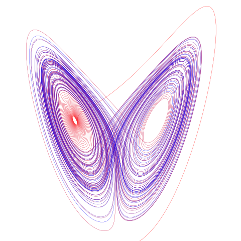
The model is a system of three different ordinary differential equations now known as the Lorenz equations, which represent the movement of a point (x, y, z) in space over time. t represents time, σ, ρ, ß are constants.

Example
First we need to define the system of differential equations:
fn lorenz_attractor(_t: f64, v: &Vec<f64>) -> Vec<f64> {
    // extract coordinates from the vec
    let (x, y, z) = (v[0], v[1], v[2]);

    // Lorenz equations
    let dx_dt = SIGMA * (y - x);
    let dy_dt = x * (RHO - z) - y;
    let dz_dt = x * y - BET * z;

    // derivatives as vec
    vec![dx_dt, dy_dt, dz_dt]
}
Constants
Let's define the initial conditions of the system r₀ = (x₀, y₀, z₀), the constants σ, ρ and ß and also a time series. One normally assumes that the parameters , σ, ρ and ß are positive. Lorenz used the values σ=10, ß =8/3 and ρ=28.
Time series
Initial position in space